Standing Waves and Resonance
Throughout this chapter, we have been studying traveling waves, or waves that transport energy from one place to another. Under certain conditions, waves can bounce back and forth through a particular region, effectively becoming stationary. These are called standing waves.
Another related effect is known as resonance. In Oscillations, we defined resonance as a phenomenon in which a small-amplitude driving force could produce large-amplitude motion. Think of a child on a swing, which can be modeled as a physical pendulum. Relatively small-amplitude pushes by a parent can produce large-amplitude swings. Sometimes this resonance is good—for example, when producing music with a stringed instrument. At other times, the effects can be devastating, such as the collapse of a building during an earthquake. In the case of standing waves, the relatively large amplitude standing waves are produced by the superposition of smaller amplitude component waves.
Standing Waves
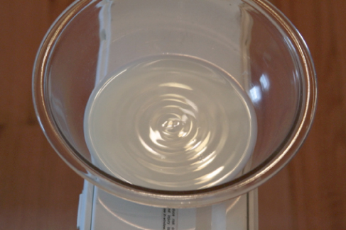
Sometimes waves do not seem to move; rather, they just vibrate in place. You can see unmoving waves on the surface of a glass of milk in a refrigerator, for example. Vibrations from the refrigerator motor create waves on the milk that oscillate up and down but do not seem to move across the surface. Figure 16.6.1 shows an experiment you can try at home. Take a bowl of milk and place it on a common box fan. Vibrations from the fan will produce circular standing waves in the milk. The waves are visible in the photo due to the reflection from a lamp. These waves are formed by the superposition of two or more traveling waves, such as illustrated in Figure 16.6.2 for two identical waves moving in opposite directions. The waves move through each other with their disturbances adding as they go by. If the two waves have the same amplitude and wavelength, then they alternate between constructive and destructive interference. The resultant looks like a wave standing in place and, thus, is called a standing wave.
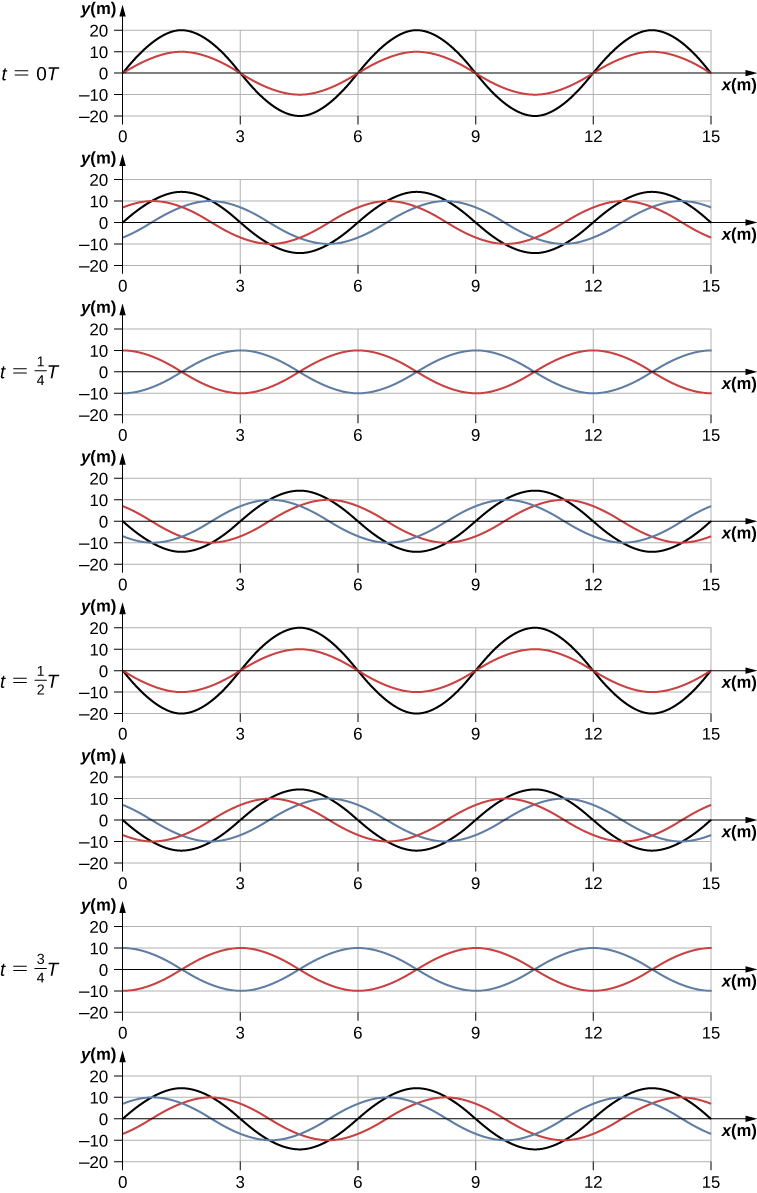 x-direction and the blue wave is moving in the +x-direction. The resulting wave is shown in black. Consider the resultant wave at the points x=0\,\text{m},3\,\text{m},6\,\text{m},9\,\text{m},12\,\text{m},15\,\text{m} and notice that the resultant wave always equals zero at these points, no matter what the time is. These points are known as fixed points (nodes). In between each two nodes is an antinode, a place where the medium oscillates with an amplitude equal to the sum of the amplitudes of the individual waves." loading="lazy"/>
Consider two identical waves that move in opposite directions. The first wave has a wave function of {y}_{1}(x,t)=A\,\text{sin}(kx-\omega t) and the second wave has a wave function {y}_{2}(x,t)=A\,\text{sin}(kx+\omega t). The waves interfere and form a resultant wave
\begin{aligned}y(x,t)={y}_{1}(x,t)+{y}_{2}(x,t), \\ y(x,t)=A\,\text{sin}(kx-\omega t)+A\,\text{sin}(kx+\omega t).\end{aligned}This can be simplified using the trigonometric identity
\text{sin}(\alpha\pm\beta)=\text{sin}\,\alpha\,\text{cos}\,\beta\pm\text{cos}\,\alpha\,\text{sin}\,\beta,where \alpha=kx and \beta=\omega t, giving us
y(x,t)=A[\text{sin}(kx)\text{cos}(\omega t)-\text{cos}(kx)\text{sin}(\omega t)+\text{sin}(kx)\text{cos}(\omega t)+\text{cos}(kx)\text{sin}(\omega t)],which simplifies to
y(x,t)=[2A\,\text{sin}(kx)]\text{cos}(\omega t).Notice that the resultant wave is a sine wave that is a function only of position, multiplied by a cosine function that is a function only of time. Graphs of y(x,t) as a function of x for various times are shown in Figure 16.6.2. The red wave moves in the negative x-direction, the blue wave moves in the positive x-direction, and the black wave is the sum of the two waves. As the red and blue waves move through each other, they move in and out of constructive interference and destructive interference.
Initially, at time t=0, the two waves are in phase, and the result is a wave that is twice the amplitude of the individual waves. The waves are also in phase at the time t=\frac{T}{2}. In fact, the waves are in phase at any integer multiple of half of a period:
t=n\frac{T}{2}\,\text{where}\,n=0,1,2,3\text{...}.\,\text{(in phase)}.At other times, the two waves are US180^\circ(\pi\,\text{radians}) out of phase, and the resulting wave is equal to zero. This happens at
t=\frac{1}{4}T,\frac{3}{4}T,\frac{5}{4}T\text{,...},\frac{n}{4}T\,\text{where}\,n=1,3,5\text{...}.\,\text{(out of phase)}.Notice that some x-positions of the resultant wave are always zero no matter what the phase relationship is. These positions are called nodes. Where do the nodes occur? Consider the solution to the sum of the two waves
y(x,t)=[2A\,\text{sin}(kx)]\text{cos}(\omega t).Finding the positions where the sine function equals zero provides the positions of the nodes.
\begin{aligned}\text{sin}(kx) & = & 0 \\ kx & = & 0,\pi,2\pi,3\pi\text{,...} \\ \frac{2\pi}{\lambda}x & = & 0,\pi,2\pi,3\pi\text{,...} \\ x & = & 0,\frac{\lambda}{2},\lambda,\frac{3\lambda}{2}\text{,...}=n\frac{\lambda}{2}\quad n=0,1,2,3\text{,...}.\end{aligned}There are also positions where y oscillates between y=\pm A. These are the antinodes. We can find them by considering which values of x result in \text{sin}(kx)=\pm1.
\begin{aligned}\text{sin}(kx) & = & \pm1 \\ kx & = & \frac{\pi}{2},\frac{3\pi}{2},\frac{5\pi}{2}\text{,...} \\ \frac{2\pi}{\lambda}x & = & \frac{\pi}{2},\frac{3\pi}{2},\frac{5\pi}{2}\text{,...} \\ x & = & \frac{\lambda}{4},\frac{3\lambda}{4},\frac{5\lambda}{4}\text{,...}=n\frac{\lambda}{4}\quad n=1,3,5\text{,...}.\end{aligned}What results is a standing wave as shown in Figure 16.6.3, which shows snapshots of the resulting wave of two identical waves moving in opposite directions. The resulting wave appears to be a sine wave with nodes at integer multiples of half wavelengths. The antinodes oscillate between y=\pm2A due to the cosine term, \text{cos}(\omega t), which oscillates between \pm1.
The resultant wave appears to be standing still, with no apparent movement in the x-direction, although it is composed of one wave function moving in the positive, whereas the second wave is moving in the negative x-direction. Figure 16.6.3 shows various snapshots of the resulting wave. The nodes are marked with red dots while the antinodes are marked with blue dots.
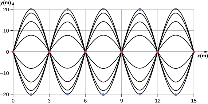 y=\pm A. The nodes are marked with red dots and the antinodes are marked with blue dots." loading="lazy"/>
A common example of standing waves are the waves produced by stringed musical instruments. When the string is plucked, pulses travel along the string in opposite directions. The ends of the strings are fixed in place, so nodes appear at the ends of the strings—the boundary conditions of the system, regulating the resonant frequencies in the strings. The resonance produced on a string instrument can be modeled in a physics lab using the apparatus shown in Figure 16.6.4.
 L. The hanging mass provides the tension in the string, and the speed of the waves on the string is proportional to the square root of the tension divided by the linear mass density." loading="lazy"/>
The lab setup shows a string attached to a string vibrator, which oscillates the string with an adjustable frequency f. The other end of the string passes over a frictionless pulley and is tied to a hanging mass. The magnitude of the tension in the string is equal to the weight of the hanging mass. The string has a constant linear density (mass per length) \mu and the speed at which a wave travels down the string equals v=\sqrt{\frac{ {F}_{T} }{\mu} }=\sqrt{\frac{mg}{\mu} }. The symmetrical boundary conditions (a node at each end) dictate the possible frequencies that can excite standing waves. Starting from a frequency of zero and slowly increasing the frequency, the first mode n=1 appears as shown in Figure 16.6.5. The first mode, also called the fundamental mode or the first harmonic, shows half of a wavelength has formed, so the wavelength is equal to twice the length between the nodes {\lambda}_{1}=2L. The fundamental frequency, or first harmonic frequency, that drives this mode is
{f}_{1}=\frac{v}{ {\lambda}_{1} }=\frac{v}{2L},where the speed of the wave is v=\sqrt{\frac{ {F}_{T} }{\mu} }. Keeping the tension constant and increasing the frequency leads to the second harmonic or the n=2 mode. This mode is a full wavelength {\lambda}_{2}=L and the frequency is twice the fundamental frequency:
{f}_{2}=\frac{v}{ {\lambda}_{2} }=\frac{v}{L}=2{f}_{1}.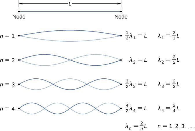 L. A node occurs at each end of the string. The nodes are boundary conditions that limit the possible frequencies that excite standing waves. (Note that the amplitudes of the oscillations have been kept constant for visualization. The standing wave patterns possible on the string are known as the normal modes. Conducting this experiment in the lab would result in a decrease in amplitude as the frequency increases.)" loading="lazy"/>
The next two modes, or the third and fourth harmonics, have wavelengths of {\lambda}_{3}=\frac{2}{3}L and {\lambda}_{4}=\frac{2}{4}L, driven by frequencies of {f}_{3}=\frac{3v}{2L}=3{f}_{1} and {f}_{4}=\frac{4v}{2L}=4{f}_{1}. All frequencies above the frequency {f}_{1} are known as the overtones. The equations for the wavelength and the frequency can be summarized as:
Register to read the full text
This page shows only part of the content. Register or log in to read it all.
Register / Log in